Reading and Taking Values From a .csv File in Matlab

Introduction

Recently, I came beyond a quote about Julia:

"Walks similar python. Runs like C."

The to a higher place line tells a lot most why I chose to write this article. I came across Julia a while ago even though information technology was in its early stages, it was still creating ripples in the numerical computing space. Julia is a work direct out of MIT, a high-level language that has a syntax as friendly as Python and functioning as competitive as C. This is non all,  It provides a sophisticated compiler, distributed parallel execution, numerical accuracy, and an all-encompassing mathematical function library.

Just this article isn't about praising Julia, information technology is about how can you utilize it in your workflow as a data scientist without going through hours of confusion which usually comes when we come up beyond a new language. Read more almost Why Julia? here.

Table of Contents

1. Installation
2. Nuts of Julia for Data Analysis
   1. Running your first plan
   2. Julia Data Structures
   3. Loops, Conditionals in Julia
3. Exploratory analysis with Julia
   1. Introduction to DataFrames.jl
   2. Visualisation in Julia using Plots.jl
   3. Bonus – Interactive visualizations using Plotly
4. Data Munging in Julia
5. Building a predictive ML model
   1. Logistic Regression
   2. Decision Tree
   3. Random Forest
6. Calling R and Python libraries in Julia
   1. Using pandas with Julia
   2. Using ggplot2 in Julia

Installation

Before we tin start our journey into the world of Julia, we need to ready our environment with the necessary tools and libraries for data science.

Installing Julia

1. Download Julia for your specific system from here

https://julialang.org/downloads/

2. Follow the platform-specific instructions to install Julia on your system from hither

https://julialang.org/downloads/platform.html

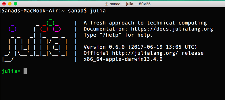
3. If you have done everything correctly, you'll get a Julia prompt from the concluding.

Installing IJulia and Jupyter Notebook

Jupyter notebook has get an environs of choice for data science since it is really useful for both fast experimenting and documenting your steps. There are other environments also for Julia like Juno IDE but I recommend to stick with the notebook. Let's look at how we can setup the same for Julia.

Go to the Julia prompt and type the following code

          julia> Pkg.add together("IJulia")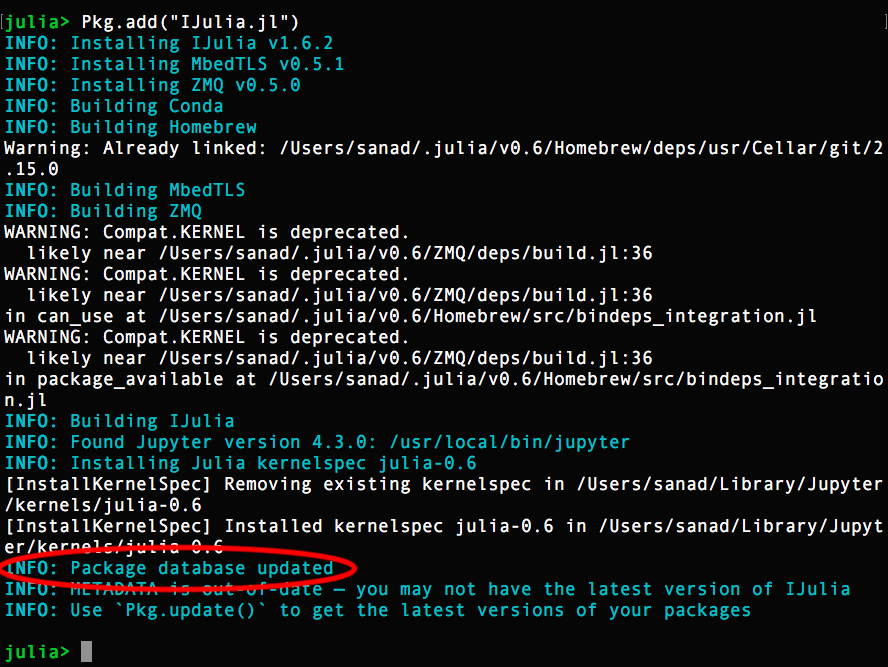

Notethat Pkg.add together() control downloads files and package dependencies in the background and installs it for you. For this, you lot should accept an active internet connection. If your internet is deadening, you lot might take to await for some time.

After ijulia is successfully installed you can blazon the following code to run it,

          julia> using IJulia   julia> notebook()

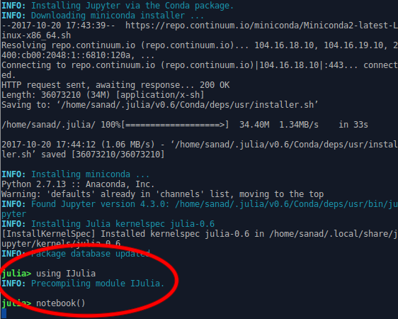
Past default, the notebook "dashboard" opens in your home directory ( homedir() ), but yous can open the dashboard in a different directory with notebook(dir="/some/path") .

There yous have your environment all set up. Let's install some important Julia libraries that we'd be needing for this tutorial.

Installing Julia Packages

A simple way of installing whatsoever package in Julia is using the command Pkg.add(".."). Like Python or R, Julia too has a long list of packages for information science. I thought instead of installing all the packages together it would be improve if we install them every bit and when needed, that'd give yous a skilful sense of what each packet does. And so nosotros will be following that process for this article.

Basics of Julia for Data Analysis

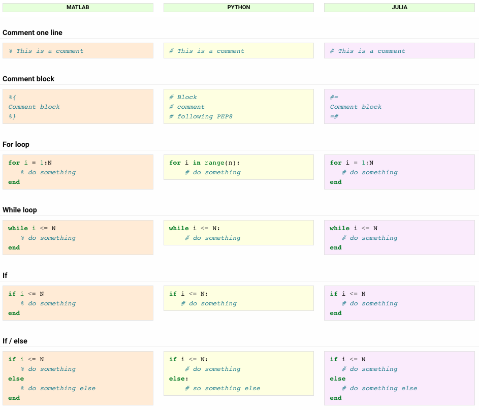
Julia is a linguistic communication that derives a lot of syntax from other information analysis tools like R, Python, and MATLAB. If you lot are from one of these backgrounds, it would take you no time to get started with information technology. Let'south learn some of the basic syntaxes. If you are in a hurry here's a cheat sheet comparing syntax of all the three languages:

          https://cheatsheets.quantecon.org/        

Running your first Julia program

1. Open up your Jupyter notebook from Julia prompt using the following control

          julia> using IJulia         julia> notebook()

2. Click on New and select Julia notebook from the dropdown

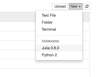
At that place, you lot created your first Julia notebook! Just like you utilise jupyter notebook for R or Python, you lot tin can write Julia code here, railroad train your models, make plots and so much more all while existence in the familiar environment of jupyter.

Few things to notation

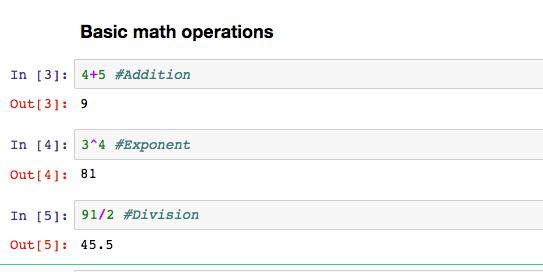
• You can name a notebook past simply clicking on the name – Untitled in the top left surface area of the notebook. The interface shows In [*] for inputs and Out[*] for output.
• You can execute a code by pressing "Shift + Enter" or "ALT + Enter", if you want to insert an additional row after.

Go alee and play around a bit with the notebook to get familiar.

Julia Information Structures

The following are some of the most common data structures we end upwardly using when performing data assay on Julia:

1. Vector(Array) – A vector is a ane-Dimensional array. A vector tin be created past merely writing numbers separated by a comma in foursquare brackets. If you add a semicolon, it volition change the row. Vectors are widely used in linear algebra.

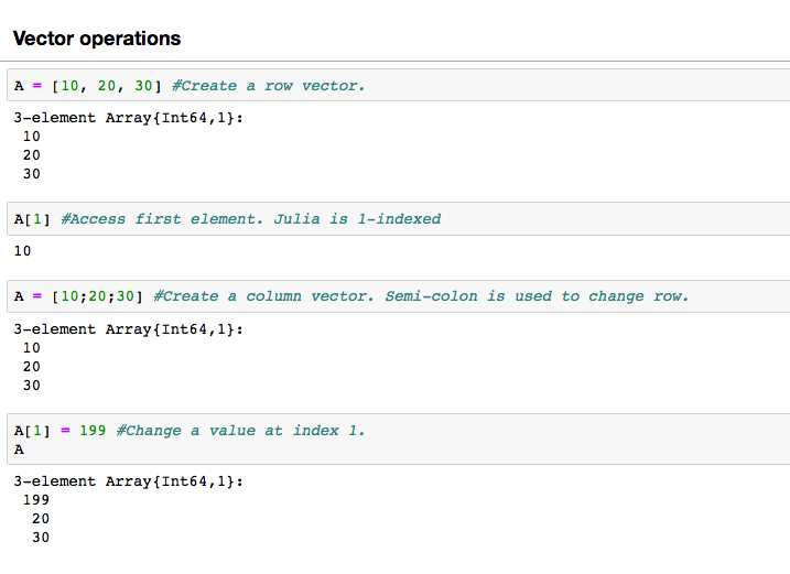
Note that in Julia the indexing starts from 1, then if you want to access the first element of an assortment you'll exercise A[1].

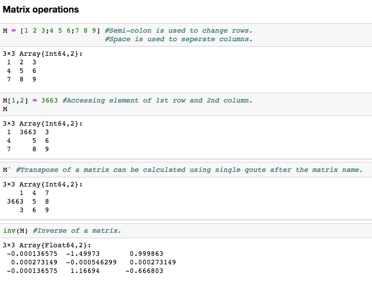
2. Matrix – Another data construction that is widely used in linear algebra, it can be thought of as a multidimensional array. Hither are some bones operations that can be performed in a matrix

3. Dictionary – D ictionary is an unordered set up of key: value pairs, with the requirement that the keys are unique (within one dictionary). You can create a lexicon using the Dict() office.

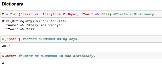
Notice that "=>" operator is used to link key with their corresponding values. You access the values of the dictionary using its key.

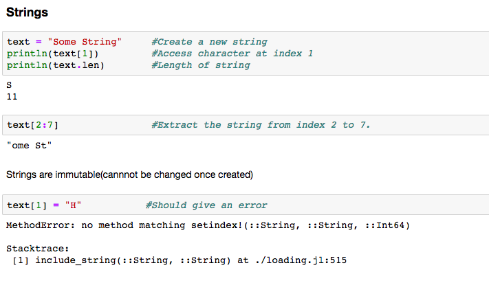
4. String – Strings can simply be defined by utilise of double ( " ) or triple ( "' ) inverted commas. Like Python, strings in Julia are also immutable(they tin can't be changed once created). Look at the error below.

Loops, Conditionals in Julia

Like virtually languages, Julia also has a FOR-loop which is the well-nigh widely used method for iteration. Information technology has a simple syntax:

          for i in [Julia Iterable]      expression(i)   end

Here "Julia Iterable" can be a vector, cord or other advanced data structures which we will explore in later sections. Let's take a look at a uncomplicated example, determining the factorial of a number 'n'.

          fact=ane   for i in range(1,5)       fact = fact*i   stop   print(fact)

Julia also supports the while loop and various conditionals like if, if/else, for selecting a bunch of statements over some other based on the outcome of the condition. Here is an example,

          if N>=0        print("N is positive")    else        print("N is negative")    terminate

The higher up lawmaking snippet performs a check on N and prints whether it is a positive or a negative number. Note that julia is non indentation sensitive like Python simply it is a practiced exercise to indent your code that'due south why you'll detect code samples in this article well indented. Hither is a list of Julia conditional constructs compared to their counterparts in MATLAB and Python.

You can learn more nigh Julia basics here .

At present that nosotros are familiar with Julia fundamentals, permit's have a deep dive into problem-solving. Yes, I hateful making a predictive model! In the process, nosotros utilise some powerful libraries and besides come across the side by side level of data structures. Nosotros will take you through the 3 central phases:

1. Information Exploration – finding out more than nigh the data nosotros have
2. Information Munging – cleaning the data and playing with it to make it better suit statistical modeling
3. Predictive Modeling – running the bodily algorithms and having fun 🙂

Exploratory Analysis using Julia (Analytics Vidhya Hackathon)

The first step in any kind of information analysis is exploring the dataset at mitt. There are two means to do that, the beginning is exploring the data tables and applying statistical methods to find patterns in numbers and the 2d is plotting the data to find patterns visually.

The onetime requires an avant-garde data structure that is capable of handling multiple operations and at the same time is fast and scalable. Like many other data assay tools, Julia provides one such construction called DataFrame. Yous need to install the following package for using it:

          julia> Pkg.add together("DataFrames.jl")        

Introduction to DataFrames.jl

A dataframe is similar to Excel workbook – you have cavalcade names referring to columns and y'all have rows, which tin can be accessed with the use of row numbers. The essential divergence is that column names and row numbers are known as column and row alphabetize, in case of dataframes . This is similar to pandas.DataFrame in Python or data.tabular array in R.

Let's work with a real problem. We are going to analyze an Analytics Vidhya Hackathon as a practice dataset.

Practise dataset: Loan Prediction Problem

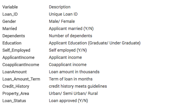
You can download the dataset from here . Here is the description of variables:

Importing libraries and the data set

In Julia we import a library by the following command:

          using <library_name>

Allow'southward outset import our DataFrames.jl library and load the railroad train.csv file of the information ready:

          using DataFrames    railroad train = readtable("railroad train.csv")

Quick Data Exploration

Once the data set is loaded, we exercise preliminary exploration on it. Such equally finding the size(number of rows and columns) of the data fix, the name of columns etc. The function size(train) is used to get the number of rows and columns of the data prepare and names(train) is used to go the names of columns(features).

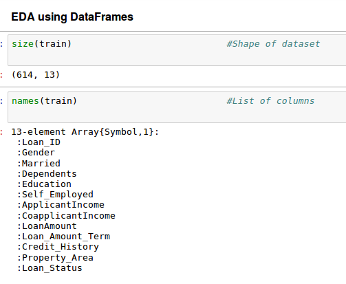
The data set is not that large(only 614 rows) knowing the size of data set sometimes affect the choice of our algorithm. There are 13 columns(features) nosotros have that is also not much, in case of a large number of features we get for techniques similar dimensionality reduction etc. Let's look at the showtime 10 rows to get a ameliorate experience of how our data looks similar? The head(,n) function is used to read the commencement n rows of a dataset.

          head(train, 10)

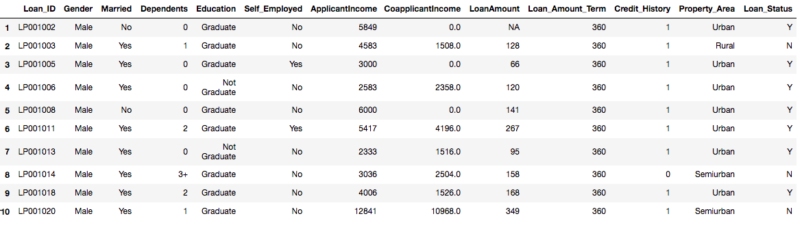
A number of preliminary inferences tin can be drawn from the higher up table such as:

• Gender, Married, Teaching, Self_Employed, Credit_History, Property_Area are all categorical variables with 2 categories each.
• Loan_ID is just a unique number, information technology doesn't provide whatever information to help in regard to the loan getting accustomed or not.
• Some columns accept missing values similar LoanAmount.

Notation that these inferences are just preliminary they will either get rejected or updated afterwards further exploration.

I am interested in analyzing the LoanAmount column, let's have a closer expect at that.

          describe(train[:LoanAmount])

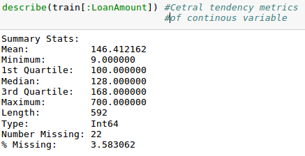
describe() part would provide the count(length), mean, median, minimum, quartiles and maximum in its output (Read this article to refresh basic statistics to sympathize population distribution).

Please annotation that we tin get an idea of a possible skew in the data by comparing the mean to the median, i.e. the 50% figure.

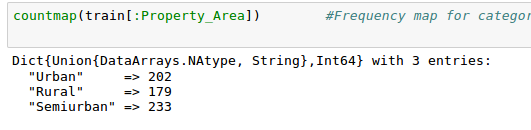
For the non-numerical values (e.g. Property_Area, Credit_History etc.), we can look at frequency distribution to sympathise whether they brand sense or not. The frequency table can exist printed by the following control:

          countmap  (  train[:Property_Area])

Similarly, we can look at unique values of credit history. Note that dataframe_name[:column_name] is a bones indexing technique to admission a particular cavalcade of the dataframe. A column can likewise be accessed past its index. For more than information, refer to the documentation .

Visualisation in Julia using Plots.jl

Another effective way of exploring the data is by doing it visually using diverse kind of plots as information technology is rightly said, "A motion picture is worth a thousand words" .

Julia doesn't provide a plotting library of its own but information technology lets yous use whatsoever plotting library of your own choice in Julia programs. In social club to use this functionality you need to install the following package:

          julia> Pkg.add("Plots.jl")   julia>Pkg.add("StatPlots.jl")   julia>Pkg.add("PyPlot.jl")

The package "Plots.jl" provides a unmarried frontend(interface) for any plotting library(matplotlib, plotly, etc.) you want to use in Julia. "StatPlots.jl" is a supporting package used for Plots.jl. "PyPlot.jl" is used to work with matplotlib of Python in Julia.

Distribution assay

Now that we are familiar with basic data characteristics, let us study the distribution of various variables. Permit us start with numeric variables – namely ApplicantIncome and LoanAmount

Let's start past plotting the histogram of ApplicantIncome using the following commands:

          using Plots, StatPlots     #import required packages   pyplot()                   #Set the backend as matplotlib.pyplot   Plots.histogram(dropna(train[:ApplicantIncome]),bins=50,xlabel="ApplicantIncome",labels="Frequency")                       #Plot histogram

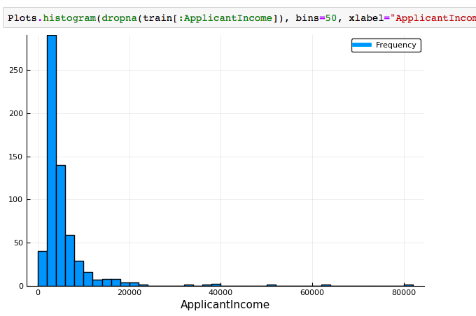
Here we observe that in that location are few extreme values. This is also the reason why fifty bins are required to depict the distribution clearly.

Next, we look at box plots to understand the distributions. Box plot for fare can exist plotted by:

          Plots.boxplot(dropna(train[:ApplicantIncome]), xlabel="ApplicantIncome")

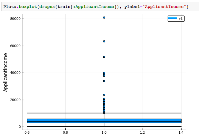
This confirms the presence of a lot of outliers/farthermost values. This tin be attributed to the income disparity in the guild. Office of this can exist driven by the fact that we are looking at people with different education levels. Let united states segregate them by Education:

          Plots.boxplot(railroad train[:Education],train[:ApplicantIncome],labels="ApplicantIncome")

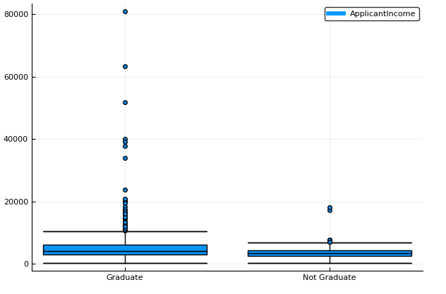
We can see that there is no substantial difference betwixt the mean income of graduate and not-graduates. But there are a higher number of graduates with very high incomes, which are appearing to be the outliers.

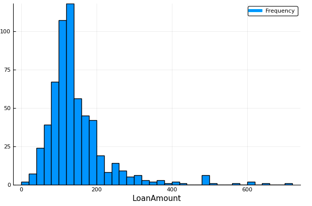
Now, Let's expect at the histogram and boxplot of LoanAmount using the following command:

          Plots.histogram(dropna(train[:LoanAmount]),bins=50,xlabel="LoanAmount",labels="Frequency")

          Plots.boxplot(dropna(train[:LoanAmount]), ylabel="LoanAmount")

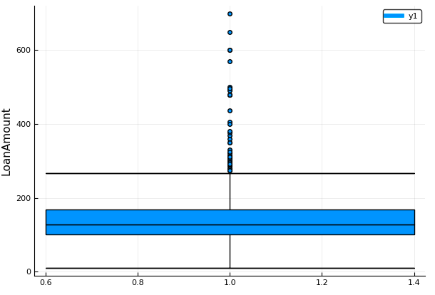
Once more, there are some extreme values. Clearly, both ApplicantIncome and LoanAmount crave some amount of information munging. LoanAmount has missing and well every bit extreme values, while ApplicantIncome has a few extreme values, which demand deeper understanding. We will take this up in coming sections.

That was a lot of useful visualizations, to acquire more than about creating visualizations in Julia using Plots.jl Plots.jl Documentation

Bonus: Interactive visualizations using Plotly

Now's the time where awesomeness of Plots.jl comes into play. The visualizations we created till now were all good but while exploration information technology is useful if the plot is interactive. We tin can create interactive plots in Julia using Plotly as a backend. Type the following code

          plotly()  #apply plotly equally backend   Plots.histogram(dropna(train[:ApplicantIncome]),bins=l,xlabel="ApplicantIncome",labels="Frequency")

Y'all can do much more with Plots.jl and various backends it supports. Read Plots.jl Documentation 🙂

Data Munging in Julia

For those, who have been following, hither yous must wear your shoes to get-go running.

Data munging – recap of the need

While our exploration of the data, we found a few bug in the data set up, which needs to be solved before the data is prepare for a practiced model. This exercise is typically referred equally "Data Munging". Here are the bug, we are already enlightened of:

1. There are missing values for some variables. We should estimate those values wisely depending on a number of missing values and the expected importance of variables.
2. While looking at the distributions, we saw that ApplicantIncome and LoanAmount seemed to contain extreme values at either stop. Though they might make intuitive sense, but should be treated accordingly.

In improver to these problems with numerical fields, we should also look at the not-numerical fields i.e. Gender, Property_Area, Married, Education and Dependents to see, if they comprise any useful information.

Check missing values in the dataset

Let us look at missing values in all the variables considering about of the models don't work with missing data and even if they do, imputing them helps by and large. So, let us check the number of nulls / NaNs in the dataset

          showcols(train)

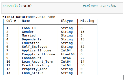
Though the missing values are not very high in number, many variables take them and each one of these should be estimated and added to the data.

Note: Remember that missing values may not always be NaNs. For case, if the Loan_Amount_Term is 0, does it makes sense or would you consider that missing? I suppose your answer is missing and you're correct. So we should bank check for values which are unpractical.

How to fill missing values?

There are multiple means of fixing missing values in a dataset. Have LoanAmount for case, at that place are numerous ways to fill up the missing values – the simplest being replacement by the mean.

The other extreme would be to build a supervised learning model to predict loan corporeality on the footing of other variables and then use historic period along with other variables to predict survival.

We would exist taking the simpler arroyo to set missing values in this article:

          #replace missing loan corporeality with hateful of loan amount railroad train[isna.(train[:LoanAmount]),:LoanAmount] = floor(mean(dropna(train[:LoanAmount]))) #replace 0.0 of loan amount with the hateful of loan amount   train[railroad train[:LoanAmount] .== 0, :LoanAmount] = floor(mean(dropna(train[:LoanAmount])))  #replace missing gender with mode of gender values  train[isna.(train[:Gender]), :Gender] = mode(dropna(train[:Gender])) #supercede missing married with mode value    railroad train[isna.(train[:Married]), :Married] = mode(dropna(railroad train[:Married]))   #supersede missing number of dependents with the way value  train[isna.(train[:Dependents]),:Dependents]=style(dropna(train[:Dependents]))   #replace missing values of the self_employed cavalcade with mode  train[isna.(train[:Self_Employed]),:Self_Employed]=mode(dropna(train[:Self_Employed]))   #supercede missing values of loan amount term with style value  train[isna.(train[:Loan_Amount_Term]),:Loan_Amount_Term]=mode(dropna(railroad train[:Loan_Amount_Term])) #replace credit history missing values with way    train[isna.(train[:Credit_History]), :Credit_History] = mode(dropna(train[:Credit_History]))

I accept basically replaced all missing values in numerical columns with their ways and with the mode in categorical columns. Let's understand the code picayune closely,

          train[isna.(train[:LoanAmount]),:LoanAmount] = floor(mean(dropna(train[:LoanAmount])))

• railroad train[:LoanAmount] – access LoanAmount column from dataframe.
• isna.(..) – returns true or false based on whether there is missing value in the column.
• train[condition, :column_name] – returns the rows of the given column that satisfy the status(In this case if the values is NA).
• dropna(..) – ignore NA values.
• hateful(..) – hateful of column values.
• floor(..) – perform floor operation on the value.

I promise this gives you a better understanding of the code office that is used to fix missing values.

Equally discussed earlier, there are better ways to perform information imputation and I encourage you to learn as many as you can. Go a detailed view of different imputation techniques through this article .

Building a predictive ML model

Now that nosotros have fixed all missing values, we will be edifice a predictive machine learning model. Nosotros will as well be cross-validating it and saving it to the deejay for futurity use. The following packages are required for doing so:

          julia> Pkg.add("ScikitLearn.jl")

This packet is an interface to Python's scikit-learn package and then python users are in for a treat. The interesting matter well-nigh using this package is yous get to utilize the aforementioned models and functionality as you used in Python.

Label Encoding categorical data

Sklearn requires all data to exist of numeric blazon so let's label encode our data,

          using ScikitLearn   @sk_import preprocessing: LabelEncoder   labelencoder = LabelEncoder()   categories = [2 3 4 five 6 12 13]    for col in categories       railroad train[col] = fit_transform!(labelencoder, train[col])   end

Those who have used sklearn before volition detect this code to be familiar, nosotros are using LabelEncoder to encode the categories. I have used the alphabetize of columns with categorical data.

Next, we will import the required modules. And then we will define a generic classification part, which takes a model as input and determines the Accuracy and Cantankerous-Validation scores. Since this is an introductory article and julia code is very similar to python, I will not go into the details of coding. Please refer to this commodity for getting details of the algorithms with R and Python codes. Also, it'll be good to get a refresher on cantankerous-validation through this commodity , as information technology is a very important mensurate of ability performance.

          using ScikitLearn: fit!, predict, @sk_import, fit_transform!   @sk_import preprocessing: LabelEncoder   @sk_import model_selection: cross_val_score    @sk_import metrics: accuracy_score   @sk_import linear_model: LogisticRegression   @sk_import ensemble: RandomForestClassifier   @sk_import tree: DecisionTreeClassifier    function classification_model(model, predictors)       y = convert(Array, train[:xiii])       Ten = convert(Array, train[predictors])       X2 = convert(Assortment, test[predictors])                             #Fit the model:       fit!(model, X, y)        #Make predictions on grooming set:       predictions = predict(model, X)        #Print accuracy       accurateness = accuracy_score(predictions, y)       println("\naccuracy: ",accuracy)        #v fold cross validation       cross_score = cross_val_score(model, 10, y, cv=five)            #print cross_val_score       println("cross_validation_score: ", hateful(cross_score))        #render predictions       fit!(model, 10, y)       pred = predict(model, X2)       return pred   end

Logistic Regression

Allow's brand our beginning Logistic Regression model. One way would exist to take all the variables into the model simply this might outcome in overfitting (don't worry if you lot're unaware of this terminology still). In simple words, taking all variables might result in the model agreement complex relations specific to the data and will not generalize well. Read more about Logistic Regression .

We tin can easily make some intuitive hypothesis to gear up the ball rolling. The chances of getting a loan volition be higher for:

1. Applicants having a credit history (recall nosotros observed this in exploration?)
2. Applicants with higher applicant and co-applicant incomes
3. Applicants with higher educational activity level
4. Backdrop in urban areas with high growth perspectives

So let's make our first model with 'Credit_History'.

model = LogisticRegression() predictor_var = [:Credit_History] classification_model(model, predictor_var)

Accuracy : eighty.945% Cross-Validation Score : 80.957%

#Nosotros can try a different combination of variables: predictor_var = [:Credit_History, :Education, :Married, :Self_Employed, :Property_Area] classification_model(model, predictor_var)

Accurateness : 80.945% Cross-Validation Score : lxxx.957%

More often than not, we expect the accuracy to increment by adding variables. But this is a more than challenging example. The accurateness and cross-validation score are non getting impacted by less important variables. Credit_History is dominating the mode. We have two options now:

1. Characteristic Technology derives new information and tries to predict those. I will get out this to your inventiveness.
2. Better modeling techniques. Let's explore this next.

Decision Tree

A decision tree is some other method for making a predictive model. Information technology is known to provide higher accuracy than logistic regression model. Read more than well-nigh Conclusion Copse.

model = DecisionTreeClassifier() predictor_var = [:Credit_History, :Gender, :Married, :Didactics] classification_model(model, predictor_var)

Accuracy : fourscore.945% Cross-Validation Score : 76.656%

Here the model based on categorical variables is unable to have an touch because Credit History is dominating over them. Let's effort a few numerical variables:

#We can try different combinations of variables: predictor_var = [:Credit_History, :Loan_Amount_Term] classification_model(model, predictor_var)

Accuracy : 99.345% Cross-Validation Score : 72.009%

Here we observed that although the accuracy went up on adding variables, the cross-validation fault went down. This is the event of model over-plumbing fixtures the data. Let's try an even more than sophisticated algorithm and come across if it helps:

Random Wood

Random forest is another algorithm for solving the classification trouble. Read more about Random Forest.

An advantage with Random Forest is that nosotros tin make it work with all the features and information technology returns a feature importance matrix which can be used to select features.

model = RandomForestClassifier(n_estimators=100) predictors =[:Gender, :Married, :Dependents, :Education,  :Self_Employed, :Loan_Amount_Term, :Credit_History, :Property_Area,  :LoanAmount] classification_model(model, predictors)

Accuracy : 100.000% Cross-Validation Score : 78.179%

Here we see that the accuracy is 100% for the training prepare. This is the ultimate instance of overfitting and can be resolved in ii ways:

1. Reducing the number of predictors
2. Tuning the model parameters

The updated code would now exist

model = RandomForestClassifier(n_estimators=100, min_samples_split=25, max_depth=8, n_jobs=-1) predictors = [:ApplicantIncome, :CoapplicantIncome, :LoanAmount, :Credit_History, :Loan_Amoun_Term, :Gender, :Dependents] classification_model(model, predictors)

Accurateness : 82.410% Cross-Validation Score : 80.635%

Notice that although accuracy reduced, the cross-validation score is improving showing that the model is generalizing well. Call up that random wood models are non exactly repeatable. Different runs will result in slight variations because of randomization. But the output should stay in the ballpark.

You lot would have noticed that fifty-fifty after some bones parameter tuning on the random woods, we accept reached a cross-validation accurateness only slightly better than the original logistic regression model. This exercise gives us some very interesting and unique learning:

1. Using a more sophisticated model does not guarantee better results.
2. Avoid using circuitous modeling techniques as a black box without understanding the underlying concepts. Doing then would increase the tendency of overfitting thus making your models less interpretable
3. Feature Technology is the cardinal to success. Everyone can use Xgboost models but the existent art and creativity lie in enhancing your features to better adjust the model.

Then are y'all ready to accept on the challenge? Start your data scientific discipline journey with Loan Prediction Problem.

Calling R and Python libraries in Julia

Julia is a powerful language with interesting libraries but information technology may so happen that you want to use library of your own from outside Julia. 1 such reason can be lack of functionality in existing Julia libraries(it is still very young). For situations like this, Julia provides ways to call libraries from R and Python. Allow's see how can we do that?

Using pandas with Julia

Install the post-obit packet:

julia> Pkg.add("PyCall.jl")

using PyCall @pyimport pandas as pd df = pd.read_csv("railroad train.csv")

There is something interesting about using a Python library every bit smoothly in another language.

Pandas is a very mature and performant library, it is certainly a bliss that we can use it wherever the native DataFrames.jl falls short.

Using ggplot2 in Julia

Install the following packages:

julia> Pkg.add("RDatsets.jl") julia> Pkg.add together("RCall.jl")

using RCall, RDatasets  mtcars = datasets("datasets", "mtcars"); library(ggplot2) ggplot($mtcars, aes(x = WT, y=MPG)) + geom_point()

End Notes

I hope this tutorial will aid you maximize your efficiency when starting with data science in Julia. I am sure this not but gave yous an thought well-nigh bones data analysis methods but information technology also showed you how to implement some of the more sophisticated techniques available today.

Julia is actually a great tool and is condign an increasingly popular language among the data scientists. The reason beingness, information technology's piece of cake to learn, integrates well with other tools, gives C like speed and likewise allows using libraries of existing tools like R and Python.

So, learn Julia to perform the full life-cycle of any information science project. Information technology includes reading, analyzing, visualizing and finally making predictions.

Also note, all the lawmaking used in this commodity is bachelor on GitHub.

If you come up across any difficulty while practicing Julia, or you have any thoughts/suggestions/feedback on the post, please feel free to mail them in comments below.

Learn, engage, compete, and get hired!

mullinstwereper.blogspot.com

Source: https://www.analyticsvidhya.com/blog/2017/10/comprehensive-tutorial-learn-data-science-julia-from-scratch/